Decision Trees - Regression

Regression Decision Trees are very similar to Classification Decision Trees, just switching the target variable type from categorical to numerical. In this section, we are going to Regression Decision Trees using same features as classfication predicting wage instead of success in order to validate the results of Classification Decision Trees.

import pandas as pd
import numpy as np
import seaborn as sns
import matplotlib.pyplot as plt
from sklearn.tree import DecisionTreeRegressor
from sklearn.ensemble import RandomForestRegressor
from sklearn.model_selection import train_test_split
from sklearn.metrics import mean_squared_error

sns.set_theme(palette="Set2")

acs = pd.read_csv("./data/acs_cleaned.csv")

acs['NATIVITY'] = acs['NATIVITY'].astype('category')
acs['DECADE'] = acs['DECADE'].astype('category')
acs['ENG'] = acs['ENG'].astype('category')
acs['MAR'] = acs['MAR'].astype('category')
acs['RAC1P'] = acs['RAC1P'].astype('category')
acs['SEX'] = acs['SEX'].astype('category')
acs['ESR'] = acs['ESR'].astype('category')
acs['SCHL'] = acs['SCHL'].astype('category')
acs['SUCCESS'] = acs['SUCCESS'].astype('category')

immigrants = acs[acs["NATIVITY"]==2]
natives = acs[acs["NATIVITY"]==1]

immigrant_X = immigrants.drop(["NATIVITY","POBP","SCHL","WAGP",'SUCCESS'], axis=1)
immigrant_y = immigrants['SUCCESS']

natives_X = natives.drop(["NATIVITY","POBP","SCHL","WAGP",'SUCCESS'], axis=1)
natives_y = natives['SUCCESS']

immigrant_X.head()

	DECADE	ENG	MAR	RAC1P	SEX	ESR	AGEP
17	5	2	3	1	2	1	47
26	5	4	2	1	2	6	87
64	5	0	5	1	2	6	59
168	4	2	5	6	1	6	55
192	6	3	5	8	2	6	61

---

Base Tree Model

Immigrants

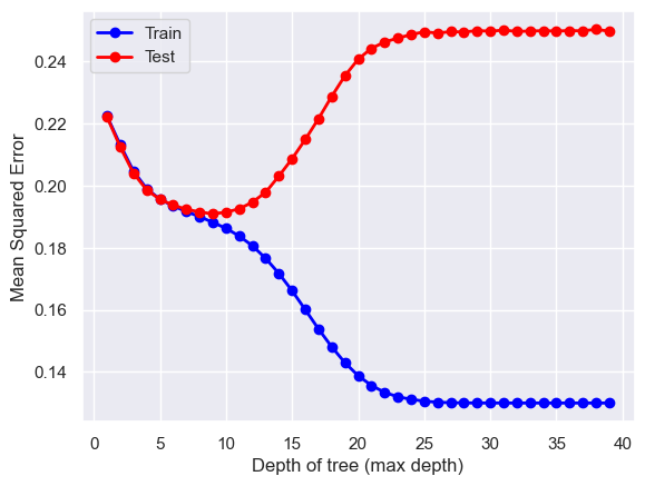
x_train, x_test, y_train, y_test = train_test_split(immigrant_X, immigrant_y,  test_size=0.2, random_state=0)

# HYPER PARAMETER SEARCH FOR OPTIMAL NUMBER OF NEIGHBORS 
hyper_param=[]
train_error=[]
test_error=[]

# LOOP OVER HYPER-PARAM
for i in range(1,40):
    # INITIALIZE MODEL 
    model = DecisionTreeRegressor(max_depth=i)

    # TRAIN MODEL 
    model.fit(x_train,y_train)

    # OUTPUT PREDICTIONS FOR TRAINING AND TEST SET 
    yp_train = model.predict(x_train)
    yp_test = model.predict(x_test)

    # shift=1+np.min(y_train) #add shift to remove division by zero 
    err1=mean_squared_error(y_train, yp_train) 
    err2=mean_squared_error(y_test, yp_test) 

    hyper_param.append(i)
    train_error.append(err1)
    test_error.append(err2)
        
plt.plot(hyper_param,train_error ,linewidth=2, marker = 'o', color='blue', label = "Train")
plt.plot(hyper_param,test_error ,linewidth=2, marker = 'o', color='red', label = "Test")
plt.legend()
plt.xlabel("Depth of tree (max depth)")
plt.ylabel("Mean Squared Error")
plt.show()

The optimal number of max_depth is 9.

model1 = DecisionTreeRegressor(max_depth=hyper_param[np.argmin(test_error)]).fit(x_train,y_train)
print("Train MSE:",mean_squared_error(y_train,model1.predict(x_train)))
print("Test MSE:",mean_squared_error(y_test,model1.predict(x_test)))

Train MSE: 0.18811852829164444
Test MSE: 0.1908230597280799

Native-borns

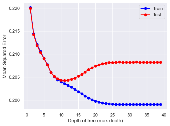
x_train, x_test, y_train, y_test = train_test_split(natives_X, natives_y,  test_size=0.2, random_state=0)

# HYPER PARAMETER SEARCH FOR OPTIMAL NUMBER OF NEIGHBORS 
hyper_param=[]
train_error=[]
test_error=[]

# LOOP OVER HYPER-PARAM
for i in range(1,40):
    # INITIALIZE MODEL 
    model = DecisionTreeRegressor(max_depth=i)

    # TRAIN MODEL 
    model.fit(x_train,y_train)

    # OUTPUT PREDICTIONS FOR TRAINING AND TEST SET 
    yp_train = model.predict(x_train)
    yp_test = model.predict(x_test)

    # shift=1+np.min(y_train) #add shift to remove division by zero 
    err1=mean_squared_error(y_train, yp_train) 
    err2=mean_squared_error(y_test, yp_test) 

    hyper_param.append(i)
    train_error.append(err1)
    test_error.append(err2)
        
plt.plot(hyper_param,train_error ,linewidth=2, marker = 'o', color='blue', label = "Train")
plt.plot(hyper_param,test_error ,linewidth=2, marker = 'o', color='red', label = "Test")
plt.legend()
plt.xlabel("Depth of tree (max depth)")
plt.ylabel("Mean Squared Error")
plt.show()

The optimal number of max_depth is 11.

model2 = DecisionTreeRegressor(max_depth=hyper_param[np.argmin(test_error)]).fit(x_train,y_train)
print("Train MSE:",mean_squared_error(y_train,model1.predict(x_train)))
print("Test MSE:",mean_squared_error(y_test,model1.predict(x_test)))

Train MSE: 0.22808431239460508
Test MSE: 0.22801254259500794

Random Forest

Immigrants

x_train, x_test, y_train, y_test = train_test_split(immigrant_X, immigrant_y,  test_size=0.2, random_state=0)
model3 = RandomForestRegressor(max_features='sqrt').fit(x_train,y_train)
print("Train MSE:",mean_squared_error(y_train,model3.predict(x_train)))
print("Test MSE:",mean_squared_error(y_test,model3.predict(x_test)))

Train MSE: 0.13530947242684196
Test MSE: 0.2178022141406163

Native-borns

x_train, x_test, y_train, y_test = train_test_split(natives_X, natives_y,  test_size=0.2, random_state=0)
model4 = RandomForestRegressor(max_features='sqrt').fit(x_train,y_train)
print("Train MSE:",mean_squared_error(y_train,model4.predict(x_train)))
print("Test MSE:",mean_squared_error(y_test,model4.predict(x_test)))

Train MSE: 0.19942831337814032
Test MSE: 0.20608541607388628

Results

Predicting wage had a similar pattern from Classification Decision Trees. There was no significant improvement on Random Forests compared to base Decision Trees in terms of MSE. In predicting immigrants’ wage, Random Forests rather got increased MSE from 0.19 to 0.22. Only in native-borns’ data, Random Forests decreased its MSE from 0.23 to 0.21, yet it is a very small difference.

data = {
    "Decision Tree (Immigrants)": model1.feature_importances_,
    "Decision Tree (Native-borns)": model2.feature_importances_,
    "Random Forest (Immigrants)": model3.feature_importances_,
    "Random Forest (Native-borns)": model4.feature_importances_,
}
df = pd.DataFrame(data).transpose()
df.columns = immigrant_X.columns
df

	DECADE	ENG	MAR	RAC1P	SEX	ESR	AGEP
Decision Tree (Immigrants)	0.038212	0.448709	0.022826	0.277486	0.009005	0.127535	0.076227
Decision Tree (Native-borns)	0.005165	0.015377	0.166531	0.130345	0.047975	0.377689	0.256918
Random Forest (Immigrants)	0.083918	0.184460	0.048860	0.145045	0.018059	0.071230	0.448427
Random Forest (Native-borns)	0.019876	0.022016	0.159436	0.128245	0.028079	0.284065	0.358282

In important features, Regression Decision Trees had different features than Classification Decision Trees, even though the success label was based on the wage. In Decision Trees of immigrants, ENG, RAC1P, and ESR were the top 3 inmporant features. This is completely different from native-born data having ESR, AGEP, and MARas their top 3. Random forests also have different results. From immigrants’ data, AGEP, ENG, and RAC1P were the top 3, but AGEP, ESR, and MAR were the top 3 from native-borns’ data.