Association Rule Mining (ARM) is a data science technique aimed at discovering interesting relationships, patterns, or associations within the datasets. Using a transaction data examining co-occurrence and frequency of features, it identifies hidden patterns, dependencies, and correlations in the data. This connection between features are visualized in a network graph which is easy to interpret.
Data Preparation
# Import necessary librariesimport pandas as pdimport numpy as npimport seaborn as snsimport matplotlib.pyplot as pltimport networkx as nx from apyori import aprioriimport warnings# Suppress warnings for cleaner outputwarnings.filterwarnings("ignore")# Load the ACS data from the provided CSV fileacs = pd.read_csv("./data/acs_cleaned.csv")# Convert specific columns to categorical types for better memory usage and analysisacs['NATIVITY'] = acs['NATIVITY'].astype("category")acs['DECADE'] = acs['DECADE'].astype(str)acs['ENG'] = acs['ENG'].astype(str)acs['MAR'] = acs['MAR'].astype(str)acs['RAC1P'] = acs['RAC1P'].astype(str)acs['SEX'] = acs['SEX'].astype(str)acs['ESR'] = acs['ESR'].astype(str)acs['SCHL'] = acs['SCHL'].astype(str)acs['SUCCESS'] = acs['SUCCESS'].astype(str)# Drop unnecessary columns from the DataFrameacs = acs.drop(["POBP","AGEP","WAGP"],axis=1)# Separate data into immigrants and natives based on the 'NATIVITY' columnimmigrants = acs[acs["NATIVITY"]==2].drop(["NATIVITY"],axis=1)natives = acs[acs["NATIVITY"]==1].drop(["NATIVITY"],axis=1)# Append prefixes to categorical variables in the immigrants DataFrameimmigrants['DECADE'] ="DECADE_"+ immigrants['DECADE']immigrants['ENG'] ="ENG_"+ immigrants['ENG']immigrants['MAR'] ="MAR_"+ immigrants['MAR']immigrants['RAC1P'] ="RACE_"+ immigrants['RAC1P']immigrants['SEX'] ="SEX_"+ immigrants['SEX']immigrants['ESR'] ="ESR_"+ immigrants['ESR']immigrants['SCHL'] ="SCHL_"+ immigrants['SCHL']# Append prefixes to categorical variables in the natives DataFramenatives['DECADE'] ="DECADE_"+ natives['DECADE']natives['ENG'] ="ENG_"+ natives['ENG']natives['MAR'] ="MAR_"+ natives['MAR']natives['RAC1P'] ="RACE_"+ natives['RAC1P']natives['SEX'] ="SEX_"+ natives['SEX']natives['ESR'] ="ESR_"+ natives['ESR']natives['SCHL'] ="SCHL_"+ natives['SCHL']# Display the first few rows of the immigrants DataFrameimmigrants.head()
DECADE
ENG
MAR
RAC1P
SEX
ESR
SCHL
SUCCESS
17
DECADE_5
ENG_2
MAR_3
RACE_1
SEX_2
ESR_1
SCHL_22
1
26
DECADE_5
ENG_4
MAR_2
RACE_1
SEX_2
ESR_6
SCHL_13
0
64
DECADE_5
ENG_0
MAR_5
RACE_1
SEX_2
ESR_6
SCHL_1
0
168
DECADE_4
ENG_2
MAR_5
RACE_6
SEX_1
ESR_6
SCHL_1
0
192
DECADE_6
ENG_3
MAR_5
RACE_8
SEX_2
ESR_6
SCHL_16
0
US Census data is splitted into immigrants’ and native-borns’ data. AGEP and WAGP columns are removed because they are numerical and POBP column are also removed because it contains too many values. Values in other columns are recoded so that each person (row) can have their own unique “transaction” so that the algorithm can interpret the connection well.
Functions
def reformat_results(results): keep = []for i inrange(0, len(results)):for j inrange(0, len(list(results[i]))):# If the index is greater than 1 (which usually represents the association rule)if (j >1):for k inrange(0, len(list(results[i][j]))):# Check if the antecedent of the rule is not emptyif (len(results[i][j][k][0]) !=0): rhs =list(results[i][j][k][0]) # Right-hand side of the rule lhs =list(results[i][j][k][1]) # Left-hand side of the rule conf =float(results[i][j][k][2]) # Confidence of the rule lift =float(results[i][j][k][3]) # Lift of the rule# Append the rule details to the 'keep' list keep.append([rhs, lhs, supp, conf, supp * conf, lift])# If the index is 1 (typically representing support), assign it to 'supp'if (j ==1): supp = results[i][j] # Support of the rule# Create a DataFrame from the collected rule informationreturn pd.DataFrame(keep, columns=["rhs", "lhs", "supp", "conf", "supp x conf", "lift"])def convert_to_network(df): G = nx.DiGraph() for row in df.iterrows(): lhs ="_".join(row[1][0]) # Joining elements of left-hand side as node name rhs ="_".join(row[1][1]) # Joining elements of right-hand side as node name conf = row[1][3] # Confidence of the rule# Add nodes to the graph if they don't already existif (lhs notin G.nodes): G.add_node(lhs)if (rhs notin G.nodes): G.add_node(rhs)# Create an edge between the LHS and RHS nodes with weight as confidence edge = (lhs, rhs)if edge notin G.edges: G.add_edge(lhs, rhs, weight=conf)# Return the created directed graphreturn Gdef plot_network(G):#SPECIFIY X-Y POSITIONS FOR PLOTTING pos=nx.spring_layout(G)#GENERATE PLOT fig, ax = plt.subplots() fig.set_size_inches(10, 10)#assign colors based on attributes weights_e = [G[u][v]['weight'] for u,v in G.edges()]#SAMPLE CMAP FOR COLORS cmap=plt.cm.get_cmap('Blues') colors_e = [cmap(G[u][v]['weight']*5.0) for u,v in G.edges()]#PLOT nx.draw( G, edgecolors="black", edge_color=colors_e, node_size=3000, linewidths=2, font_size=10, font_color="white", font_weight="bold", width=weights_e, with_labels=True, pos=pos, ax=ax ) ax.set(title='Network Graph') plt.show()
ARM
Immigrants
Code
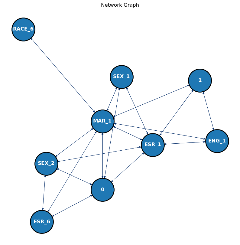
# Perform association rule mining using Apriori algorithm on the immigrants' dataresults =list(apriori(immigrants.to_numpy(), min_support=0.225, min_confidence=0.0, min_lift=0, min_length=1))# Reformat the obtained association rule mining results into a structured DataFramepd_results = reformat_results(results)# Convert the DataFrame of association rules into a directed graphG = convert_to_network(pd_results)# Plot the generated network graphplot_network(G)
Native-borns
Code
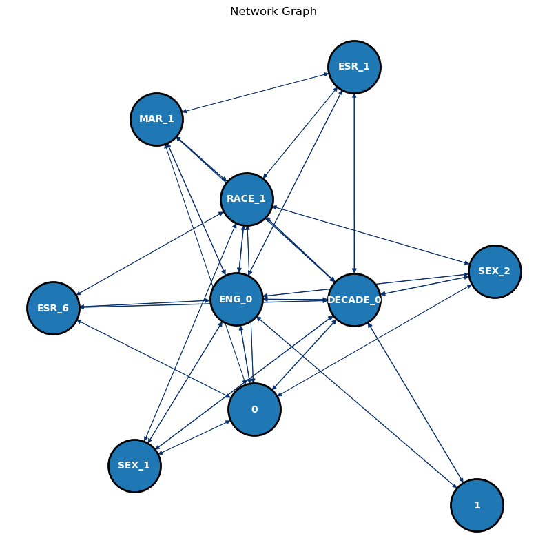
# Perform association rule mining using Apriori algorithm on the native-borns' dataresults =list(apriori(natives.to_numpy(), min_support=0.3, min_confidence=0.0, min_lift=0, min_length=1, max_length=2)) # Reformat the obtained association rule mining results into a structured DataFramepd_results = reformat_results(results)# Convert the DataFrame of association rules into a directed graphG = convert_to_network(pd_results)# Plot the generated network graphplot_network(G)
Results
The being successful(1) is highly connected with ENG_1, ESR_1, and MAR_1 in immigrants’ network graph. Among them, MAR_1 has the most connection with other features, even with not being successful(2). RACE_6 has a sole connection with MAR_1 and SEX_1, SEX_2, MAR_1, ESR_1, and ESR_6 has a connection with not being successful(2).
In the case of native-borns’ data, the networks gets a lot more complex even though the max_length is limited to 2. There is significantly less connection to being successful(1) compared to immigrants’ network graph, having only ENG_0 and DECADE_0. Not being successful(2) is connected with SEX_1, ESR_6, MAR_1, ENG_0, RACE_1, DECADE_0, and SEX_2, and ENG_0 has the most connection with other features.