Decision Trees - Classification

A Decision Tree is a non-parametric supervised machine learning model that can be applied to both classification and regression. By forming the sequential binary questions, it is very easy to interpret. Those binary questions are formed minimizing the errors. Its flexibility to adapt to any type of dataset and problem leads to overfitting, which requires an additional step of pruning to improve their accuracy.

This inclination of overfitting can be reduced by doing Random Forests model instead. Random Forests fit numerous simple tree models and predicts the target by averaging or majority voting. This aggregation brings a flexibility to deal with complex datasets and an improvement on an accuracy.

In this section, the goal is finding out which features are the most important classifying successful immigrants and natives. Also there will be a comparison between a random classifier, a simple decision tree, and a random forest model validating the result of important features.

# Import necessary libraries
import pandas as pd
import numpy as np
import seaborn as sns
import matplotlib.pyplot as plt
from sklearn import tree
from sklearn.ensemble import RandomForestClassifier
from sklearn.model_selection import train_test_split
from collections import Counter
from sklearn.metrics import accuracy_score
from sklearn.metrics import precision_score
from sklearn.metrics import recall_score

sns.set_theme(palette="Set2")
# Load the ACS data from the provided CSV file
acs = pd.read_csv("./data/acs_cleaned.csv")

# Convert specific columns to categorical types for better memory usage and analysis
acs['NATIVITY'] = acs['NATIVITY'].astype('category')
acs['DECADE'] = acs['DECADE'].astype('category')
acs['ENG'] = acs['ENG'].astype('category')
acs['MAR'] = acs['MAR'].astype('category')
acs['RAC1P'] = acs['RAC1P'].astype('category')
acs['SEX'] = acs['SEX'].astype('category')
acs['ESR'] = acs['ESR'].astype('category')
acs['SCHL'] = acs['SCHL'].astype('category')
acs['SUCCESS'] = acs['SUCCESS'].astype('category')

# Separate data into immigrants and natives based on the 'NATIVITY' column
immigrants = acs[acs["NATIVITY"]==2]
natives = acs[acs["NATIVITY"]==1]

immigrant_X = immigrants.drop(["NATIVITY","POBP","SCHL","WAGP",'SUCCESS'], axis=1)
immigrant_y = immigrants['SUCCESS']

natives_X = natives.drop(["NATIVITY","POBP","SCHL","WAGP",'SUCCESS'], axis=1)
natives_y = natives['SUCCESS']

immigrant_X.head()

	DECADE	ENG	MAR	RAC1P	SEX	ESR	AGEP
17	5	2	3	1	2	1	47
26	5	4	2	1	2	6	87
64	5	0	5	1	2	6	59
168	4	2	5	6	1	6	55
192	6	3	5	8	2	6	61

Similar to Naive Bayes section, US Census data is splitted into immigrants’ and native-borns’ data for the comparison. The WAGP and SCHL are removed because the target label SUCCESS is made from those two variables. POBP and NATIVITY variables are also removed because the data is splitted by NATIVITY and POBP is not an effective predictor. Other variables are changed to a category type from integer as they should be.

def random_classifier(y_data):
    y_pred = []
    max_label = np.max(y_data)  # Find the maximum label value in y_data
    for i in range(0, len(y_data)):
        # Generate random predictions within the range of label values
        y_pred.append(int(np.floor((max_label + 1) * np.random.uniform(0, 1))))
    
    # Display the count of predicted values and their probabilities
    print("Count of prediction:", Counter(y_pred).values())  # Counts the elements' frequency
    print("Probability of prediction:", np.fromiter(Counter(y_pred).values(), dtype=float) / len(y_data))
    
    # Calculate and display accuracy, precision, and recall scores
    print("Accuracy:", accuracy_score(y_data, y_pred))
    print("Precision:", precision_score(y_data, y_pred))
    print("Recall:", recall_score(y_data, y_pred))

def confusion_plot(y_true, y_pred, title):
    # Calculate and display accuracy, precision, and recall scores
    print("Accuracy:", accuracy_score(y_true, y_pred))
    print("Precision:", precision_score(y_true, y_pred))
    print("Recall:", recall_score(y_true, y_pred))
    
    # Create a confusion matrix using pandas crosstab and plot it as a heatmap using seaborn
    confusion_matrix = pd.crosstab(y_true, y_pred, rownames=['True'], colnames=['Predicted'])
    sns.heatmap(confusion_matrix, annot=True, fmt='d', cbar=False, cmap="Greens")
    plt.title(title)
    plt.show()

---

Random Classifier

print("Immigrants")
random_classifier(list(immigrant_y))
print("\n")
print("Native-borns")
random_classifier(list(natives_y))

Immigrants
Count of prediction: dict_values([109806, 110267])
Probability of prediction: [0.49895262 0.50104738]
Accuracy: 0.5001022388025791
Precision: 0.4167248587519385
Recall: 0.5013802660149047


Native-borns
Count of prediction: dict_values([1078897, 1079851])
Probability of prediction: [0.49977904 0.50022096]
Accuracy: 0.5002709904074029
Precision: 0.3565085453013587
Recall: 0.500070206093889

Baseline random classifier gives about 50% of accuracy. This baseline model is necessary to evaluate the effectiveness of following tree models.

Base Tree Model

Immigrants

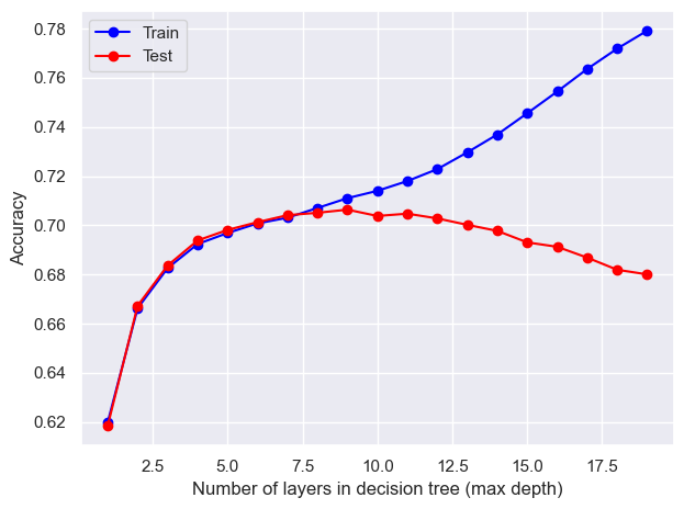
# Split the data into training and testing sets using train_test_split
x_train, x_test, y_train, y_test = train_test_split(immigrant_X, immigrant_y, test_size=0.2, random_state=0)

# Initialize empty lists to store training and testing results
test_results = []
train_results = []

# Loop through different numbers of layers (max_depth) for decision tree
for num_layer in range(1, 20):
    # Create a Decision Tree Classifier with varying max_depth  
    model = tree.DecisionTreeClassifier(max_depth=num_layer)
    model = model.fit(x_train, y_train)

    # Make predictions on training and testing sets
    yp_train = model.predict(x_train)
    yp_test = model.predict(x_test)

    # Store accuracy scores for training and testing sets at each max_depth
    test_results.append([num_layer, accuracy_score(y_test, yp_test)])
    train_results.append([num_layer, accuracy_score(y_train, yp_train)])

# Plotting the training and testing accuracy scores against the number of layers (max_depth)
plt.plot([column[0] for column in train_results], [column[1] for column in train_results], marker='o', color="blue", label="Train")
plt.plot([column[0] for column in test_results], [column[1] for column in test_results], marker='o', color="red", label="Test")
plt.ylabel("Accuracy")
plt.xlabel("Number of layers in decision tree (max depth)")
plt.legend()
plt.tight_layout()
plt.show()

The optimal number of max_depth is 9.

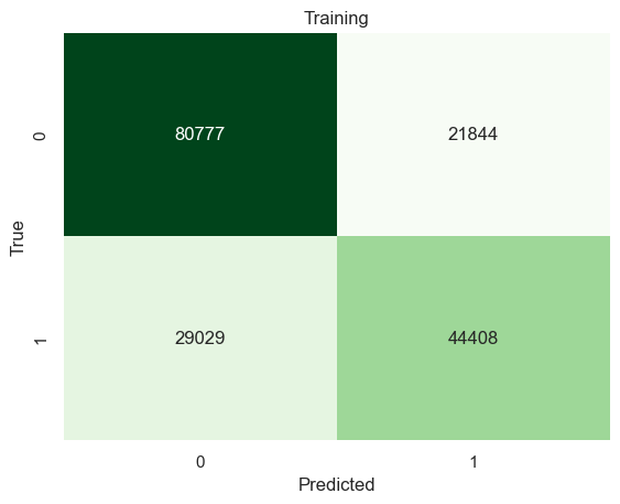
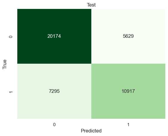
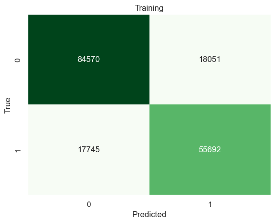
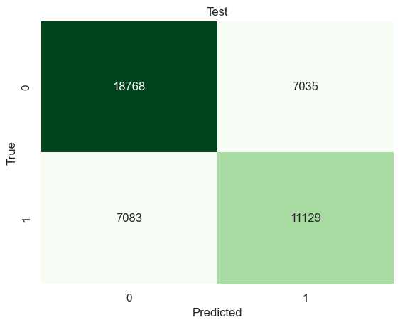
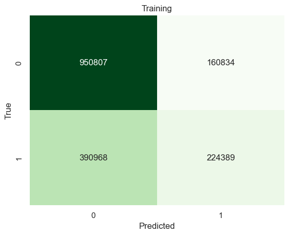
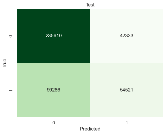
# Build a tree model using a optimal parameter
model1 = tree.DecisionTreeClassifier(max_depth=[column[0] for column in test_results][np.argmax([column[1] for column in test_results])])
model1 = model1.fit(x_train,y_train)
yp_train=model1.predict(x_train)
yp_test=model1.predict(x_test)

print("------TRAINING------")
confusion_plot(y_train,yp_train,"Training")

print("------TEST------")
confusion_plot(y_test,yp_test,"Test")

------TRAINING------
Accuracy: 0.7110440877438117
Precision: 0.6702891988166395
Recall: 0.6047087980173482
------TEST------
Accuracy: 0.7063728274451891
Precision: 0.659796929771546
Recall: 0.5994399297166704

The best decision tree model has 70% accuracy on classifying successful immigrants.

Native-borns

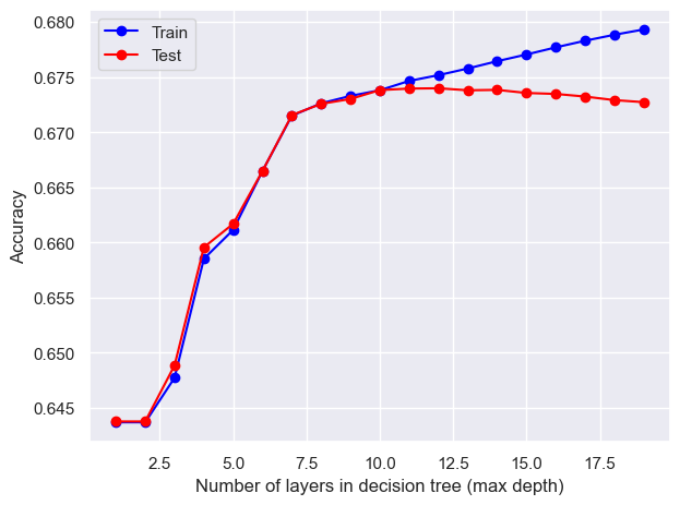
x_train, x_test, y_train, y_test = train_test_split(natives_X, natives_y,  test_size=0.2, random_state=0)

test_results=[]
train_results=[]

for num_layer in range(1,20):
    model = tree.DecisionTreeClassifier(max_depth=num_layer)
    model = model.fit(x_train,y_train)

    yp_train=model.predict(x_train)
    yp_test=model.predict(x_test)

    test_results.append([num_layer,accuracy_score(y_test, yp_test)])
    train_results.append([num_layer,accuracy_score(y_train, yp_train)])

plt.plot([column[0] for column in train_results],[column[1] for column in train_results],marker='o',color="blue",label="Train")
plt.plot([column[0] for column in test_results],[column[1] for column in test_results],marker='o',color="red",label="Test")
plt.ylabel("Accuracy")
plt.xlabel("Number of layers in decision tree (max depth)")
plt.legend()
plt.tight_layout()
plt.show()

The optimal max_depth is 12.

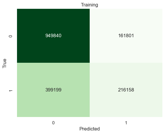
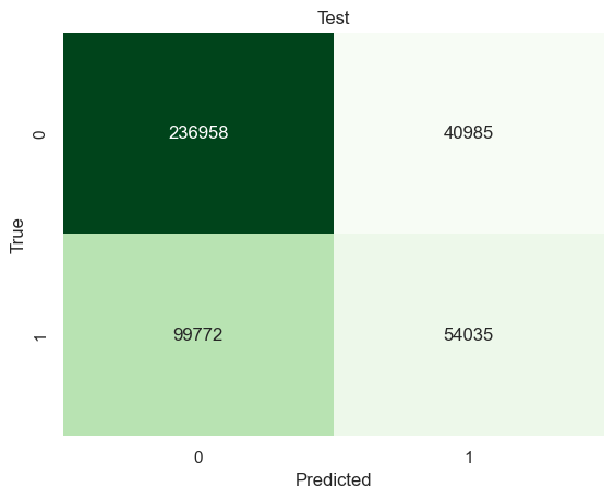
model2 = tree.DecisionTreeClassifier(max_depth=[column[0] for column in test_results][np.argmax([column[1] for column in test_results])])
model2 = model2.fit(x_train,y_train)
yp_train=model2.predict(x_train)
yp_test=model2.predict(x_test)

print("------TRAINING------")
confusion_plot(y_train,yp_train,"Training")

print("------TEST------")
confusion_plot(y_test,yp_test,"Test")

------TRAINING------
Accuracy: 0.6751588594775443
Precision: 0.5719085932601156
Recall: 0.35127251335403675
------TEST------
Accuracy: 0.6739849449913144
Precision: 0.5686697537360555
Recall: 0.3513169101536341

Random Forest

Immigrants

# Split the data into training and testing sets using train_test_split
x_train, x_test, y_train, y_test = train_test_split(immigrant_X, immigrant_y, test_size=0.2, random_state=0)

# Create and train a RandomForestClassifier with max_features set to 'sqrt' (square root of the number of features)
model3 = RandomForestClassifier(max_features='sqrt').fit(x_train, y_train)

# Make predictions on training and testing sets
yp_train = model3.predict(x_train)
yp_test = model3.predict(x_test)

# Print confusion matrices and evaluation metrics for training and testing sets
print("------TRAINING------")
confusion_plot(y_train, yp_train, "Training")  # Display confusion matrix and metrics for training set
print("------TEST------")
confusion_plot(y_test, yp_test, "Test")  # Display confusion matrix and metrics for testing set

------TRAINING------
Accuracy: 0.7966806393347646
Precision: 0.755217444367601
Recall: 0.758364312267658
------TEST------
Accuracy: 0.6792457116891969
Precision: 0.6126954415327021
Recall: 0.6110806061937184

Native-borns

x_train, x_test, y_train, y_test = train_test_split(natives_X, natives_y,  test_size=0.2, random_state=0)
model4 = RandomForestClassifier(max_features='sqrt').fit(x_train,y_train)
yp_train=model4.predict(x_train)
yp_test=model4.predict(x_test)

print("------TRAINING------")
confusion_plot(y_train,yp_train,"Training")
print("------TEST------")
confusion_plot(y_test,yp_test,"Test")

------TRAINING------
Accuracy: 0.6804848644873938
Precision: 0.5824911804331517
Recall: 0.36464848860092597
------TEST------
Accuracy: 0.671988419224088
Precision: 0.5629194457637269
Recall: 0.3544767143237954

Results

Both Decision trees and Random Forests are better than a random classifiers. Yet it is also true that there is no significant improvement on the accuracy on classifying successful immigrants or native-borns. Decision tree model got 70% and 67% accuracy on classifying successful immigrants and native-borns. Random Forests got 68% and 67% accuracy. Random Forests had no big improvement on accuracy.

data = {
    "Decision Tree (Immigrants)": model1.feature_importances_,
    "Decision Tree (Native-borns)": model2.feature_importances_,
    "Random Forest (Immigrants)": model3.feature_importances_,
    "Random Forest (Native-borns)": model4.feature_importances_,
}
df = pd.DataFrame(data).transpose()
df.columns = immigrant_X.columns
df

	DECADE	ENG	MAR	RAC1P	SEX	ESR	AGEP
Decision Tree (Immigrants)	0.008178	0.017990	0.164526	0.129104	0.047927	0.372782	0.259493
Decision Tree (Native-borns)	0.008204	0.018002	0.164509	0.129107	0.047925	0.372793	0.259460
Random Forest (Immigrants)	0.020526	0.022396	0.156595	0.131182	0.027787	0.282938	0.358575
Random Forest (Native-borns)	0.020274	0.022307	0.152880	0.129481	0.028947	0.285889	0.360221

The important features across the nativity and models are also similar. Decision trees used ENG, AGEP, MAR,and RAC1P as their top 4 most important features. And Random Forests has AGEP, ENG, MAR,and RAC1P having age as the most important fearture.