Clustering is an unsupervised machine learning technique. Rather than predicting the labels or target numbers, it discovers unseen information by forming clusters from the data.
1. KMeans Clustering
KMeans clustering is an approach that finds the k clusters based on centroids. Those centroids are “centers” of the cluster calculated by taking the mean of all distances between all points in a cluster and the centroid. For the distances, Euclidean or Manhattan distance are used. This process of assigning clusters continues until the algorithm converges having the minimum error.
2. DBSCAN
DBSCAN, Density Based Spatial Clustering of Applications with Noise, finds spaces that has the highest density around and builds clusters around. This is different from KMeans clustering that DBSCAN are not impacted by the distance between the points. This allows outliers to be their own cluster unlike KMeans clustering.
3. Agglomerative Clustering
Agglomerative Clustering, also known as Hierarchical Clustering, has two ways of creating clusters. Agglomerative method starts with assigning every single data point into their own cluster. Then it starts to merge those clusters until there is only one big clustering containing all the data points. On the other hand, divisive method starts from the one big cluster containing all points and divides the cluster until each point forms an own cluster. In the process of merging or dividing clusters, Agglomerative Clustering uses linkage function to figure out which and how to merge or divide the clusters.
In this section, those three clustering methods will be used to find the relationship between the success rate and the place of birth. This will allow us to see whether there are some differences between countries on their success rate based on the features. There will be a hyper parameter tuning for all three methods and then the comparison on their clusters along with true clusters.
Data Preparation
# Import necessary librariesimport pandas as pdimport numpy as npimport seaborn as snsimport matplotlib.pyplot as pltfrom sklearn.cluster import KMeansfrom sklearn.cluster import AgglomerativeClusteringfrom sklearn.cluster import DBSCANfrom sklearn.metrics import silhouette_scoresns.set_theme(palette="Set2")acs = pd.read_csv("./data/acs_cleaned.csv")# Replace zero values in 'WAGP' column with 2 to avoid zero values when taking the logarithmacs.loc[acs['WAGP'] ==0, 'WAGP'] =2# Create a new column 'NORM_WAGP' containing the logarithm of 'WAGP'acs["NORM_WAGP"] = np.log(acs["WAGP"])# Convert specific columns to categorical type for better memory usage and analysisacs['NATIVITY'] = acs['NATIVITY'].astype('category')acs['DECADE'] = acs['DECADE'].astype('category')acs['ENG'] = acs['ENG'].astype('category')acs['MAR'] = acs['MAR'].astype('category')acs['RAC1P'] = acs['RAC1P'].astype('category')acs['SEX'] = acs['SEX'].astype('category')acs['ESR'] = acs['ESR'].astype('category')acs['SCHL'] = acs['SCHL'].astype('category')# Filter the dataset to consider only immigrantsimmigrants = acs[acs["NATIVITY"]==2]# Create dummy variables for certain columns and drop specific columns from the dataframedf = pd.get_dummies(immigrants.drop(["POBP", "WAGP", "NATIVITY", "SCHL"], axis=1))df2 = pd.get_dummies(immigrants[["SCHL"]])# Group by 'POBP' (Place of Birth) and calculate mean for 'SCHL' (Educational Attainment) valuesdf['POBP'] = immigrants["POBP"]df2['POBP'] = immigrants["POBP"]SCHL = df2.groupby("POBP").agg("mean")SCHL = SCHL.reset_index()# Group by 'POBP' (Place of Birth) and calculate mean for other columnsX = df.groupby("POBP").agg("mean")X = X.reset_index()# Create a binary target variable 'y' based on 'SUCCESS' column valuesy = X["SUCCESS"] >0.5# Create a variable 'wagp' containing 'NORM_WAGP' column valueswagp = X["NORM_WAGP"]# Normalize 'AGEP' column values and drop unnecessary columnsX["NORM_AGEP"] = (X["AGEP"] - np.min(X["AGEP"])) / (np.max(X["AGEP"]) - np.min(X["AGEP"]))X = X.drop(["AGEP", "POBP", "SUCCESS", "NORM_WAGP"], axis=1)X.head()
DECADE_0
DECADE_1
DECADE_2
DECADE_3
DECADE_4
DECADE_5
DECADE_6
DECADE_7
DECADE_8
ENG_0
...
RAC1P_9
SEX_1
SEX_2
ESR_1
ESR_2
ESR_3
ESR_4
ESR_5
ESR_6
NORM_AGEP
0
0.0
0.004357
0.004357
0.019608
0.061002
0.276688
0.224401
0.209150
0.200436
0.087146
...
0.315904
0.485839
0.514161
0.557734
0.017429
0.065359
0.004357
0.0
0.355120
0.350466
1
0.0
0.006897
0.003448
0.020690
0.100000
0.144828
0.244828
0.313793
0.165517
0.331034
...
0.034483
0.517241
0.482759
0.641379
0.024138
0.037931
0.010345
0.0
0.286207
0.368953
2
0.0
0.003300
0.004950
0.016502
0.024752
0.024752
0.341584
0.415842
0.168317
0.099010
...
0.006601
0.480198
0.519802
0.694719
0.023102
0.056106
0.000000
0.0
0.226073
0.310732
3
0.0
0.012346
0.037037
0.037037
0.037037
0.092593
0.271605
0.296296
0.216049
0.148148
...
0.043210
0.611111
0.388889
0.654321
0.012346
0.061728
0.000000
0.0
0.271605
0.398003
4
0.0
0.000000
0.025974
0.064935
0.181818
0.324675
0.207792
0.116883
0.077922
0.324675
...
0.324675
0.415584
0.584416
0.610390
0.012987
0.038961
0.000000
0.0
0.337662
0.506213
5 rows × 37 columns
The US Census data has 12 columns with 9 categorical variables. Since these clustering methods are not applicable to categorical variables, the dataset is aggregated by the POBP column. During the process, SCHL and WAGP columns are droped and reprocessed for the cluster plotting because the SUCCESS label is based on those columns. And AGEP column is normalized so that it can have a same range with other variables.
Hyper Parameter Tuning
KMeans Clustering
Code
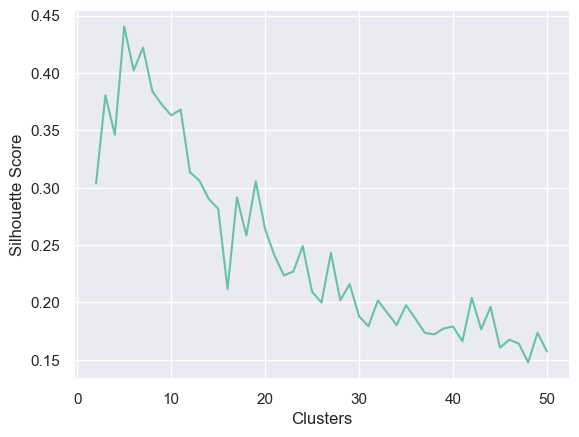
# Initialize empty lists to store silhouette scores and the number of clusterssil_score = []n_cluster = []# Loop through a range of values for KMeans clusters from 1 to 50for i inrange(1, 50): model = KMeans(n_clusters=i+1, n_init=1).fit(X)try:# Calculate silhouette score and store it along with the corresponding cluster count score = silhouette_score(X, model.labels_) n_cluster.append(i+1) sil_score.append(score)except:continue# Plot a line plot showing how silhouette score changes with different cluster countssns.lineplot(x=n_cluster, y=sil_score)plt.xlabel("Clusters")plt.ylabel("Silhouette Score")plt.show()# Find the cluster count (K) with the highest silhouette scoreprint("The silhouette score is highest when K =", n_cluster[np.argmax(sil_score)])# Fit a KMeans model using the K value with the highest silhouette scorekmeans = KMeans(n_clusters=n_cluster[np.argmax(sil_score)], n_init=1).fit(X)
The silhouette score is highest when K = 5
DBSCAN
Code
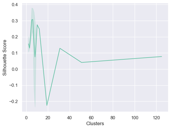
l_eps = np.arange(0.1, 2, 0.1)n_sample =range(1, 10)sil_score = []n_cluster = []best_score =0# Loop through different combinations of epsilon and minimum samplesfor eps in l_eps:for n in n_sample:# Fit DBSCAN model with varying eps and min_samples model = DBSCAN(eps=eps, min_samples=n).fit(X)try:# Calculate silhouette score and store it along with the corresponding cluster count score = silhouette_score(X, model.labels_) n_cluster.append(len(np.unique(model.labels_))) sil_score.append(score)# Update best_score and optimal parameters if a higher score is foundif score > best_score: best_score = score opt_eps = eps opt_sample = nexcept:continue# Plot a line plot showing how silhouette score changes with different cluster countssns.lineplot(x=n_cluster, y=sil_score)plt.xlabel("Clusters")plt.ylabel("Silhouette Score")plt.show() # Print the best parameters for epsilon and minimum samples and their corresponding silhouette scoreprint("The best parameters for eps and min_sample are", opt_eps, "and", opt_sample, "having the highest silhouette score of", best_score)# Fit a DBSCAN model using the optimal epsilon and minimum samplesdbscan = DBSCAN(eps=opt_eps, min_samples=opt_sample).fit(X)
The best parameters for eps and min_sample are 0.5 and 9 having the highest silhouetter score of 0.4197274085360764
Agglomerative Clustering
Code
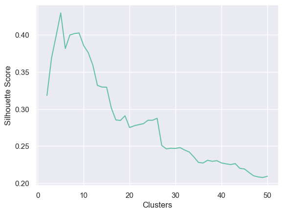
# Initialize empty lists to store silhouette scores and the number of clusterssil_score = []n_cluster = []# Loop through different numbers of clusters from 2 to 50for i inrange(2, 51):# Fit Agglomerative Clustering model with 'i' clusters model = AgglomerativeClustering(n_clusters=i).fit(X)# Obtain cluster labels from the fitted model labels = model.labels_# Calculate silhouette score and store it along with the corresponding cluster count sil_score.append(silhouette_score(X, labels)) n_cluster.append(i)# Plot a line plot showing how silhouette score changes with different cluster countsplt.plot(n_cluster, sil_score)plt.xlabel("Clusters")plt.ylabel("Silhouette Score")plt.show()# Find the cluster count (K) with the highest silhouette scoreprint("The silhouette score is highest when K =", n_cluster[np.argmax(sil_score)])# Fit an Agglomerative Clustering model using the K value with the highest silhouette scoreag = AgglomerativeClustering(n_clusters=n_cluster[np.argmax(sil_score)]).fit(X)
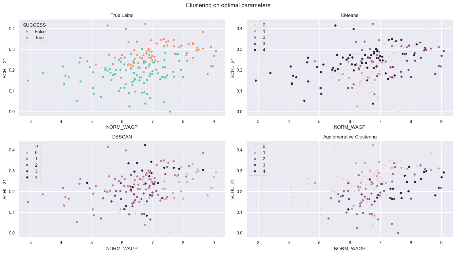
With optimal parameters, all of methods are not clustering the countries well based on their success rate. KMeans and Agglomerative Clustering have a very weak trend. In Agglomerative Clustering, ligher color coded countries are on the left and darker color countries on the right. And in KMeans, there is a cluster where ligher color coded countries are in the middle.
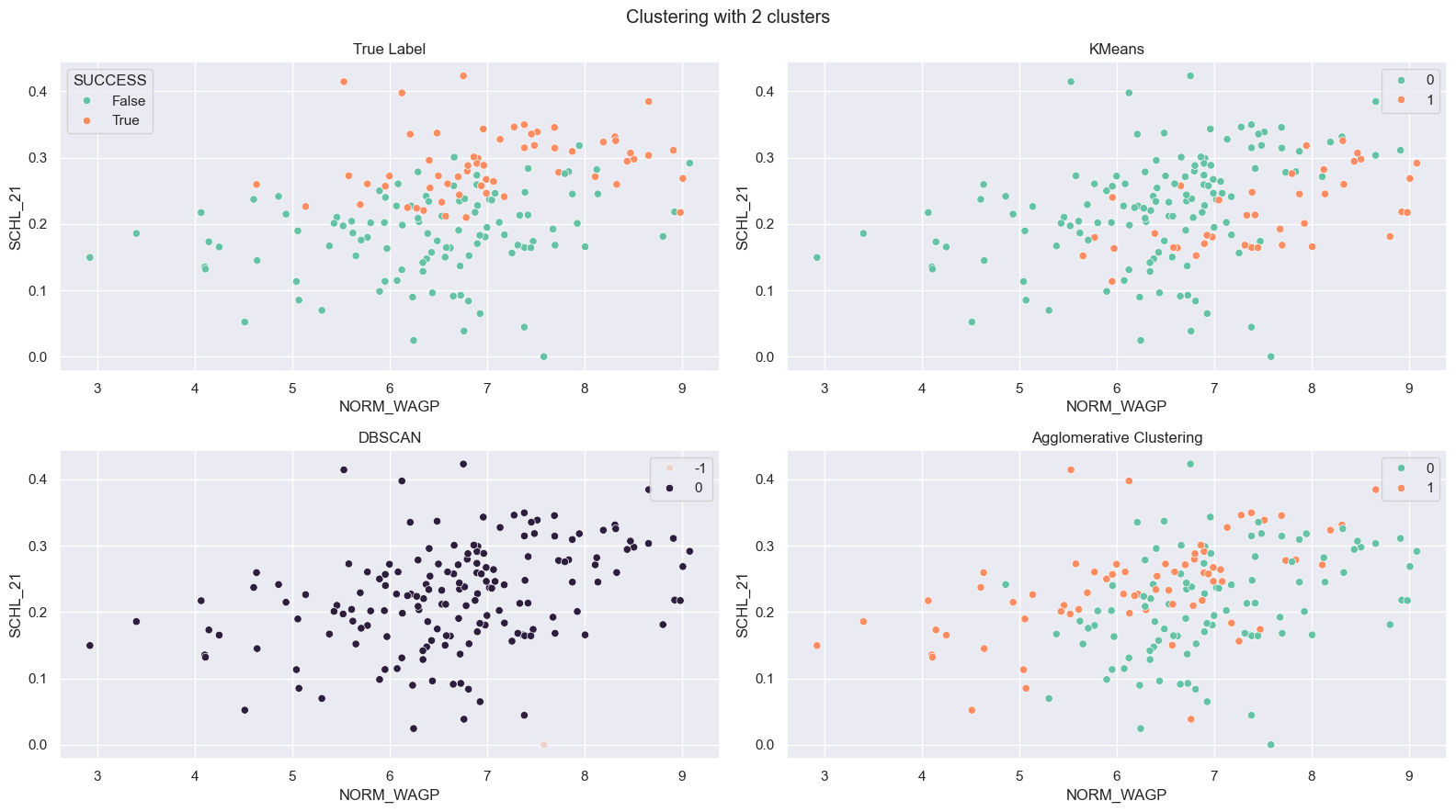
For the comparison, all three methods are forced to create only 2 clusters. KMeans and Agglomerative Clustering produce similar clusters between each other, but those clusters are still different from true cluster. DBSCAN is doing worse that clustering almost every countries into one cluster.
Results
The result is limited because the dataset is aggreagated that input data was not fully explaining the whole dataset. All three methods are failed to create clear clusters among countries on their optimal hyper parameter. This might imply that there is a no clear differences on immigrants based on their place of birth. However, when the methods are forced to create only two clusters, KMeans and Agglomerative clustering made similar clusters on the space of SCHL and normalied wage.